As it is the \( \pi \) day of the century I thought I really should write a short blog post about it.
Most people know that the first digits of pi are \( \pi = 3.141592653 \), and this year using the american format for representing the date we can get the first 9 decimal places on 3/14/15 at 9:26:53 in the morning. As I will be at #mathsconf2015 then I am going to post this post a bit early, and release it on Thursday, as most schools will celebrate pi day on the Friday before.
Since I was at school I have been pretty interested in the computation of pi, I think that this was sparked by my Year 7 maths teacher giving me a book called “The Joy of Pi” by David Blatner when he left the school.
In March 2014 David Bailey and Jonathan Borwein (famous amongst pi afficionados) wrote an article for The Mathematical Association of America about Pi Day which is well worth a read and Kate Bush even wrote a song about pi! Admittedly she gets some of the decimal digits that she sings worng….
Calculating Pi
People have been trying to calculate pi for thousands of years, the babylonians used the approximation \( \pi \approx 3.125 \) and there is evidence from the Rhind Papyrus that the Egyptian scribe Ahmes took \( \pi \) to be the ratio 256/81, or approximately 3.16049 – this is less than 1% off the true value. Pi also seems to come up in the design of the Great Pyramid at Giza; the ratio of the length of one side to the height is approximately \( \pi / 2 \).
The ancient greeks seem to have been the first to try and pin down a value of pi by a systematic means. Antiphon and Bryson of Heraclea (around 469-399 BC) used the method of exhaustion to approximate pi. They deduced that if you take a regular polygon, such as a hexagon, and keep doubling the number of sides then the limiting shape is a circle. Antiphon inscribed successive polygons inside a circle and calculated their areas, Bryson then circumscribed polygons around the cicle and compared the areas of the inscribed and circumscribed polygons. This gave an upper and a lower bound on the value of \( \pi \) since the area of a circle with radius 1 is \( \pi \). Archimedes did something similar, but instead found the circumference of inscribed and circumscribed polygons – he bounded pi between the following \( 3\frac{1}{7} < \pi < 3\frac{10}{71} \). An interactive applet of Antiphon’s and Bryson’s construction can be found here where you will see an embedded geogebra app like the following

As you can see, working out the area of a 512 sided polygon only results in upper and lower bounds that agree to 3 decimal places. Clearly people needed to find a better method….
Since the ancient greeks many people have tried to improve the number of accurate decimal digits of pi that are known, but until an improvement in the calculation algorithms happened, the number of known decimal places didn’t improve dramatically. Today, the current record was announced on 8th October 2014, where 13,300,000,000,000 decimal places were computed and verified. THe increase in the number of decimal places oer the last 600 years or so can be seen in the plot below (data taken from Wikipedia’s chronology of computation of pi page)
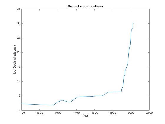
Disclaimer: This is a plot generated quickly, I’m aware that it should be a step function style plot!!
In 1621, the Dutch mathematician Willebrod Snell improved on the polygon method, and derived a better way to approximate the perimeter of a circle using a polygon of fewer sides – he was able to find pi correct to 6 decimal places using a 96 sided polygon. Things really took off though when people moved away from using polygons to calculate pi and embraced calculus. Many power series representations were discovered and employed to increase the number of decimal digits. Maybe I will write about these for pi day next year!! The Aperiodical have produced a video showing a few slowly converging methods to approximate \( \pi \)
I want to briefly examine a more modern method discovered independently by Eugene Salamin and Richard Brent in 1975, known as the Brent-Salamin algorithm. This algorithm works by computing the arithmetic-geometric mean of two specific numbers. The arithmetic mean of two numbers \(a\) and \(b\) is what people generally know as the mean, namely \(\frac{a+b}{2}\), whereas the geometric mean can be computed as \(\sqrt{ab}\). As an aside, for non-negative real numbers the arithmetic mean is always greater than or equal to the geometric mean – this is a fact we may use in some future posts discussing the analysis of finite element methods. Anyway, back to the arithmetic geometric mean algorithm: The arithmetic geometric mean or \(agm(a,b)\) is computed by repeatedly taking arithmetic and geometric means. You start with \(a_0 = a \) and \(b_0 = b \) then you keep computing the iterates
\( \begin{align*} a_{n+1} &= \frac{a_n+b_n}{2} \\ b_{n+1} &= \sqrt{a_nb_n} \end{align*} \)until your values for \(a_n\) and \(b_n\) agree to some accuracy. For example the first few iterations of the computation of the arithmetic-geometric mean of 12 and 17 produce the following
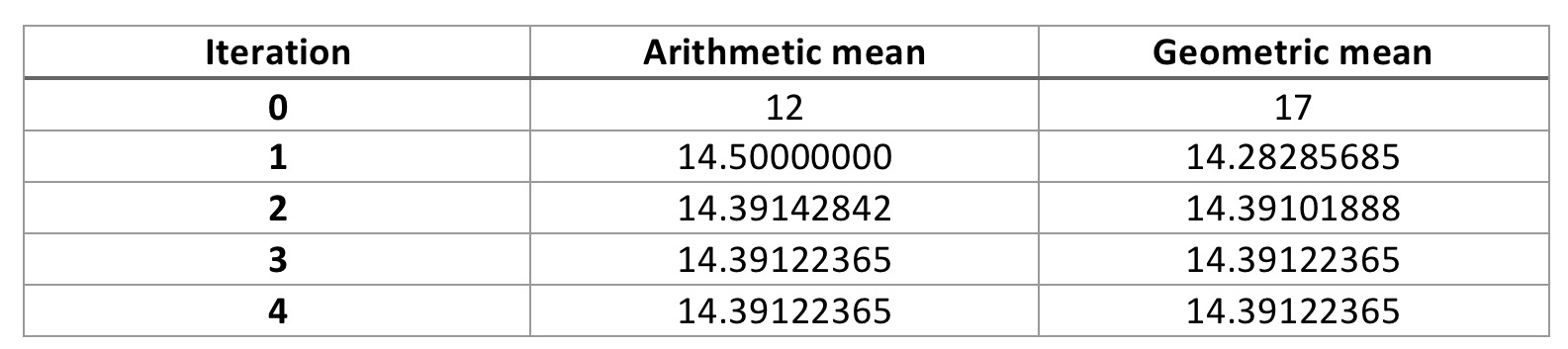
The (very simple) Matlab code to generate these numbers is here. As you can see, after only 3 iterations we have agreement to 8 decimal places, this very fast convergence (technically it is quadratic) is the reason why the agm algorithm for computing pi is so popular.
To compute \(\pi \) we set \(a = 1 \) and \( b = \frac{1}{\sqrt{2}} \), compute \( agm(a,b) \) but as we do so, in addition to computing \(a_n\) and \(b_n\) we compute \( c_n = a_{n+1} – a_n \). At the end we can then compute
\( S = \frac{1}{4} – \sum_{n=0}^{N} 2^n c_n^2, \)where \(N \) is the number of iterations we have used to compute the arithmetic-geometric mean. Finally, we can compute \( \pi \) with the following
\( \pi = \frac{(agm(a,b))^2}{S} \)In 2011 Cleve Moler, the creator of Matlab wrote a great blog post on using Matlab’s variable precision arithmetic to generate digits of pi. In this he presented an implementation of the agm algorithm, which I have modified very slighty and used to compute some digits of \( \pi \) on my laptop. The code is available here and I ran it on a mid 2013 Macbook Air with a 1.3GHz Core i5 processor with 8GB of 1600 MHz DDR3 RAM. The table below shows the number of iterations and time taken to compute a certain number of decimal digits.
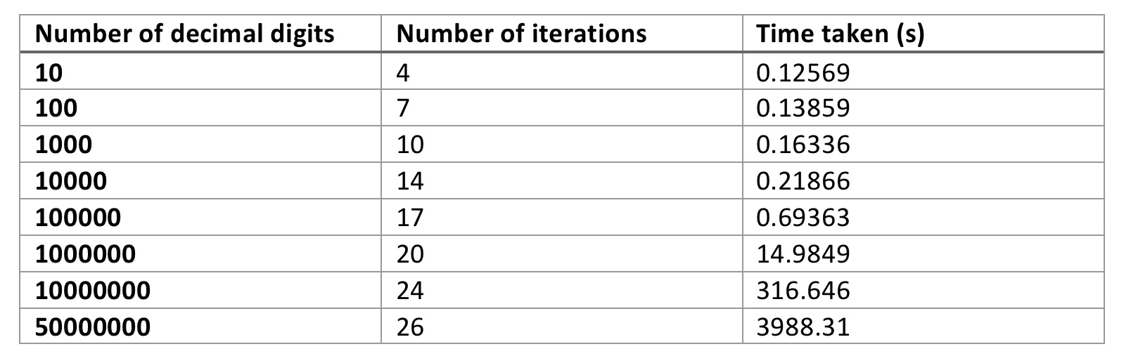
As can be seen from the table, the time taken rapidly starts to increase even though the number of iterations is growing fairly slowly. Implementing this in Matlab is obviously not the most efficient way, it would be far better (but harder) to implement it in C++ or Fortran using a robust variable precision arithmetic library. Variable precision arithmetic in itself is costly in terms of memory and computation time. As a non-scientific comparison Moler reported that computing 100000 digits took about 2.5 seconds on his laptop of the time.
The original papers of Brent and Salamin are fairly dense reads and include some elliptic integral theory which really isn’t my area. Luckily, a 1984 SIAM Review paper by Borwein and Borwein where they derive a similar iteration based on the arithmetic-geometric mean is much more accessible and is available at this link. The algorithm for computing \( \pi \) is contained in section 5; they also present algorithms for the calculation of other elementary functions.
I’m sure I will return to the problem of computing \( \pi \) on this blog in the future. Happy Pi Day!