Categories
Uncategorized

Secondary Curriculum Development Meeting

Last Wednesday (21st January 2015) I attended the first East Midlands Secondary Curriculum Development meeting of this year. These are hosted at the University of Nottingham and organised by the East Midlands West maths hub (@EM_MathsHub).

This was a great, thought provoking session about problem solving led by Dominic Hudson, from Heanor Gate Science College, with some additional input from Malcolm Swan of The Centre for Research in Mathematics Education in the School of Education at the University of Nottingham (@UoNSoE)

Dominic kicked off the session by presenting us with 4 problems and asked us to have a think about how a student would approach them. I particularly like the Matchless activity from nRich, available here which I think could promote a nice discussion on how to work out if you have enough information to solve a given problem – and with older pupils it could provide a nice opener to the world of under-determined systems in Linear Algebra. The activity concerning plane turn around times from Bowland Maths was also great, and I’m ashamed to say i hadn’t seen this one before. The activity is here and I think it would be fascinating to see how different pupils approach this task, and how long it takes them to realise that some tasks are independent of others.

I was very interested to hear Dominic talk about the week long problem solving activities that they have been trialling at Heanor this year; this is very similar to the few weeks of problem solving that we tried with Year 8 last year. It seems to have gone well from what he was saying and it’ s nice that he has shared the activities for us to try out too!

Malcolm Swan presented the following Framework for Designing a Balanced Mathematics Curriculum

IMG_0553.JPG
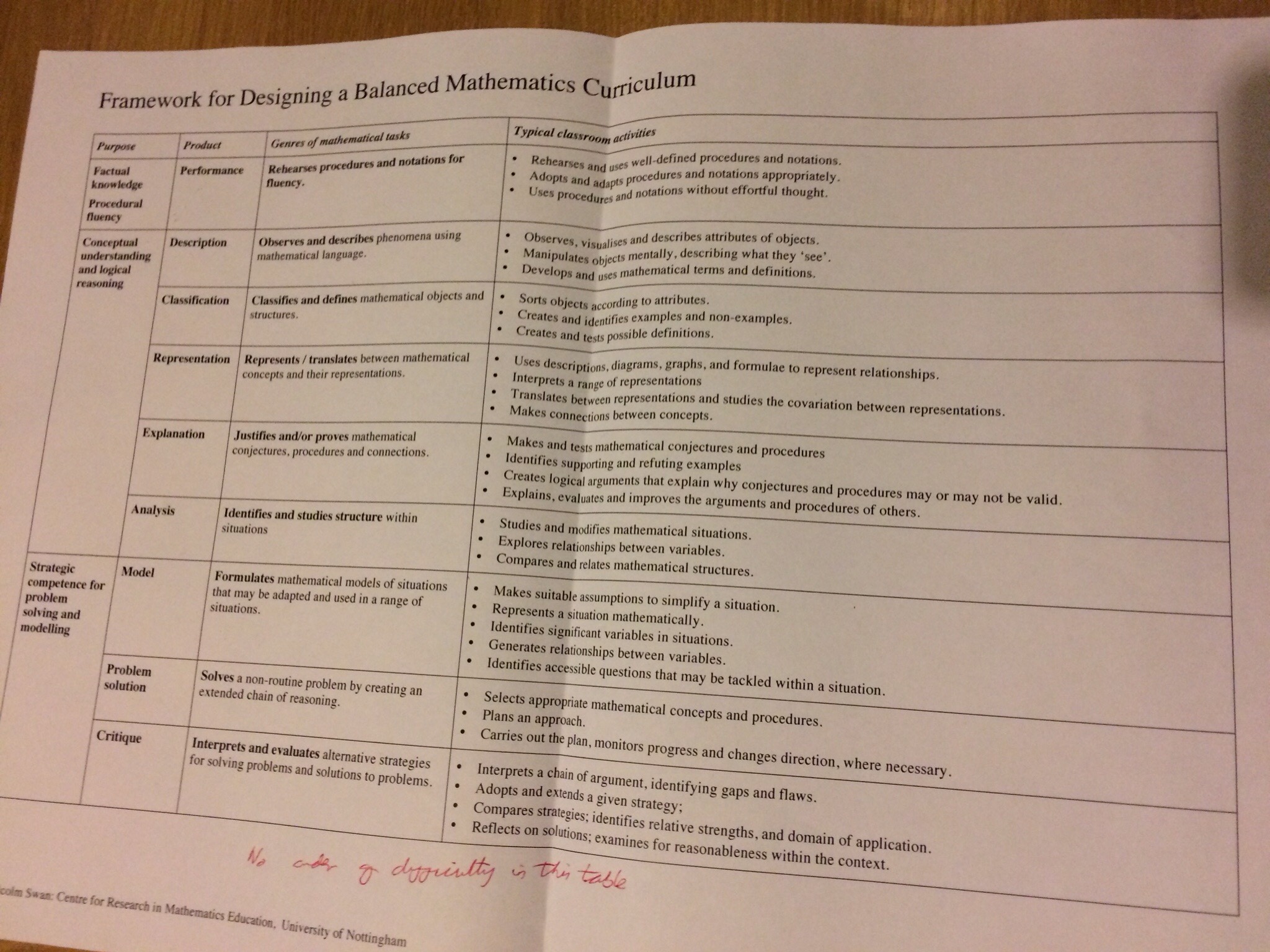
I don’t think I was alone in feeling a bit sad that in my classroom I spend a lot more time focussing on the top section of the table than on the rest. This is a real shame as the true nature of mathematics is not just becoming proficient at calculations!!
Malcolm, also gave us a copy of a conference proceeding “Designing tasks and lessons that develop conceptual understanding, strategic competence and critical awareness” from a conference talk he gave in November 2014. Unfortunately I haven’t got an electronic copy to link to here.
A key message that I took from this paper is that a problem solving exercise requires that a solution method is not known; indeed a question where a “problem” is given to be solved, but at the same time requires students to implement a given approach is an “illustrative exercise” . I immediately thought of the “Problem Solving” questions at then end of each double page spread of the new MyMaths textbooks, where it is quite clear that the questions are normally no more than worded questions about a particular topic.
I will be trying out some of the real-life graph activities that Malcolm discusses in this paper this week with my Year 9 class (these are available from the Math Shell website here).

I really value these meetings and hope they continue for longer than just this academic year!

Categories
Uncategorized

FMSP Favourite Problems – Number 1

In a fairly shameless copy of the style of some of @srcav‘s posts where he solves a maths problem and briefly goes through his reasoning I have decided to do the same with some (easier) problems that I have recently discovered.

The Further Mathematics Support Programme (FMSP) have produced a series of 6 posters of problems that should be accessible to GCSE students. The first one of which is a fairly nice area problem – the poster is available here and shown below.

IMG_0551.PNG

As always, when solving any kind of geometric / visual problem I find drawing a diagram (even if there is a printed one in front of me) helpful, and I then mark on everything that I already know.

IMG_4391.JPG
Each distinct area I have labelled with a number (maybe lower case letters or greek letters would have been a better choice, but never mind!) and I now proceed to write down as much as I can quickly calculate. Here, that involves a bit of Pythagoras’ theorem and the formulae for working out the area of a right angled triangle:

IMG_4393.JPG
Now comes the slightly harder bit, where I actually had to think and work out how I could find the shaded areas that I was interested in using only what I had already worked out. It was actually fairly easy, as soon as I had written some things down!!

IMG_0552.JPG
The result is lovely, in that the area of the shaded regions is the same area as the triangle

Overall, I think this is a nice, accessible problem that would get students to think.
As, an aside this problem demonstrates (though it isn’t immediately clear from the picture) the fact that Pythagoras’ theorem can be extended for other shapes attached to the sides of a right angled triangle – in this case semi-circles.

Categories
A Level Software Teaching

Matlab in the Classroom

One of the things I have missed since teaching in a school is the fact that I don’t have access to Matlab….

Matlab is a product from The Mathworks, designed originally for numerical computation (indeed the name derives from MATrix LABoratory as the software was originally focussed towards operations on matrices) but which now is capable of much more. More information about Matlab and The Mathworks is available here.

I had got used to using Matlab in teaching an demonstrating, not least because of the ease with which you can use it to check matrix computations, plot graphs of functions and demonstrate numerical methods.

Last term I set my Year 12 Further Mathematicians some homework which involved them researching the Jacobi Method and performing 2 iterations of this method on a \(2 \times 2\) matrix system. I wanted to be able to demonstrate this straightforward numerical method to them, without having to work out how to use the Python IDE on the Windows computers at school, so I decided to give Matlab Mobile a try.

Matlab Mobile was originally released in 2010 (see here for an early blog post discussing Matlab Mobile) but I hadn’t had much reason to use it before. Originally the app needed to connect to your computer with a running copy of Matlab, but since it’s release it has become a lot better. Th app is currently on version 4.1.1 which is a universal app suitable for both the iPad and the iPhone. With this version (as long as you have a valid Matlab Licence for desktop) you can connect to a copy of Matlab running in the cloud to execute commands. You can also upload your files to the cloud so that they can be run from the app.

On opening the app you are presented with a screen that looks like this:

IMG_0538.PNG

The left hand portion of the screen displays commands that you have typed and on the right hand side you can toggle between Figures and viewing your command history.

Using a keyboard (I recommend using a bluetooth keyboard here as the on screen keyboard takes up so much space) it is easy to type short commands that accomplish complex things. For example, in the screen shot below, I create a matrix and then find its eigenvalues using the eigs command. As you can see this command can also return the corresponding eigenvectors of a matrix simply by explicitly giving two output arguments to the function.

IMG_0539-0.PNG

One of the great uses of the Matlab desktop product is to prototype functions before coding in another language. Unfortunately, the mobile app does not allow you to edit or create .m script files or function files. This is a real shame, especially as it extends to the inability to make small edits to files you have already stored in the cloud. Luckily though, you can at least view the test of functions that you have written by using the command type in the command window, as shown below.

IMG_0540-0.PNG
The code shown above is a naive implementation of the iterative Jacobi scheme for solving systems of linear equations – I stress it is not the most efficient way to code this algorithm, but it is clear for teaching purposes. Using Matlab Mobile I was able to discuss this short function with my class, and relate it to the algorithm that they had to research and then express in pseudocode.
If you are going to use Matlab Mobile for a similar purpose I would recommend avoiding writing script files and instead use function files with enough arguments to allow you to vary everything you will want to demonstrate the affect of. I would also say it is probably useful to print more of the internal workings of the function to the command line than you would normally.

Another great piece of functionality in Matlab is the ability to produce professional looking graphs with very little effort. You can still generate figures such as the one below (a visualisation of the Barnsley fern after 10000 iterations – I may write a blog post about this in the future) in the Cloud, but a lot of the data exploration tools in the figure window of the desktop product are not usable. You can however, save the figure to your camera roll or email it to yourself.

IMG_0541-0.PNG
As a final example of the graphical abilities of Matlab Mobile the 3D surface plot below was created using 4 lines of code.

IMG_0542-0.PNG

One important thing to note is that I couldn’t connect to the Matlab Cloud through my schools wifi (I suspect because of the firewall) and so had to resort to using my phone as a 4G hotspot.

All in all, if you have a Matlab licence it is well worth familiarising yourself with the Mobile app, and I managed to do all that I wanted to do in the classroom with it. I just needed to do a bit more forward planning than I would have done if I had had access to the fully fledged Matlab product! Hopefully as the app develops they will remove some of the limitations that are currently present.

Categories
Teaching

A Starter for all Groups

Sometimes I like to do a quick starter with my groups where they are just playing with numbers and which isn’t related to the work of a particular lesson.
One day last week I decided I wanted a starter that I could use across all abilities and year groups. I remembered the following problem that I had recently read on Dan Meyer’s (@ddmeyer) blog here:

  • Choose three consecutive whole numbers and add them. Write your sum on the board. What do you notice?

I chose to use this problem as it seems simple but can revel lots about the nature of numbers. The only modification I made was to restrict the numbers that could be chosen to be less than or equal to 50 – I did this to make the arithmetic manageable.

I was very happy with the response I got to this problem from all of my groups, they were all engaged with thinking about what they could say about the results, especially once they had come and written them on the whiteboard.
I found this task good for the lower attaining KS3 as a way of getting them to practice mental / written addition methods and to have a look at how to tell if a number is divisible by 3 or not. With the higher attaining students it led on to a discussion of knowing something and how to rigorously show it using algebra. We also discussed how it doesn’t matter how the consecutive numbers are labelled, we will always get a sum that is divisible by 3.

Overall I think this activity benefited my students and that it was a valuable thing to do, which I will try to repeat in future. Of course, having to plan one activity that can be used with all classes is a nice bonus in terms of planning time!

Categories
A Level Books Teaching

Classic Maths Books 1 – Bostock and Chandler textbooks

This week I posted the following picture on Twitter:

IMG_0537.JPG
A few people retweeted, favourited and commented how good they were for questions to stretch A Level students so I thought I would write a bit more here.
They were first published in 1982 and are still available from Amazon here and here.
I think I got my copies when I was doing my A Levels and asked my teacher if there were any other books he would recommend that weren’t the Edexcel ones.
I think they are still fantastic books, vastly superior to the Pearson published textbooks, though I think some students may find them a bit dry. They certainly assume more knowledge than the current books and the later questions are generally more involved (or it is less clear on how to start them). There are some really nice examples in the book, such as:

  • Find the complex roots of the equation \(2x^2 + 3x + 5 = 0 \). If these roots are \( \alpha \) and \( \beta \), confirm the relationships \( \alpha + \beta = – \frac{b}{a} \) and \( \alpha \beta = \frac{c}{a} \)

All these examples are well explained, and it is easy to follow them line by line.
One other aspect of them that I appreciate are the multiple choice questions at the end of each chapter; these are great for a quick test of understanding and I am using some of them in some QuickKey quizzes that I am trialling this half term.
I may make a blog post about a classic mathematics book a fairly regular thing… gives me an excuse to get some of the older books off my shelf again 🙂

Categories
Uncategorized

Nottingham Lakeside’s George Green Exhibition

This is a post that I should have written months ago when this exhibition opened. Unfortunately it is closing on Sunday, it’s open 12pm-4pm tomorrow and Sunday, the details are available here. If you are local to Nottingham and have some spare time it is well worth a visit.

George Green is probably one of Nottingham’s most famous residents. The science library of The University of Nottingham is named after him. He was a miller based in the Sneinton area of Nottingham, he had little formal education but published a paper (by subscription) in 1828 where he presented the following theorem, given below in modern notation.

Green’s Theorem
Let \( R \) be a simply connected plane domain whose boundary is a simple, closed, piecewise smooth curve \(C\) oriented counter-clockwise. If \( f(x,y) \) and \( g(x,y) \) are continuous and have continuous first partial derivatives on some open set containing \( R \), then


\( \int_C f(x,y) \mathrm{d}x + g(x,y) \mathrm{d}y = \int \int_R \left ( \frac{\partial g}{\partial x} – \frac{\partial f}{\partial y} \right) \mathrm{d} A
\)

This theorem has had wide ranging influences, but at the time received limited exposure due to the local nature of the publication and it not being published in a scientific journal.

An interesting fact about this paper is that Green used Leibniz’s notation for the calculus as opposed to Newton’s notation which was in common usage in England at the time.

If you want to learn more about George Green the following two videos are a good place to start:
Maths history trail of Nottingham – George Green
Sixty Symbols – George Green