This is a joint blog post by me and Jasmina Lazic, my co-presenter at #mathsconf6 (see my write up of the day) on Saturday 5th March 2016.
Me and Jasmina first interacted over twitter, and over time the idea of leading a workshop at a #mathsconf took root. Collaborating over email and a couple of WebEx calls we came up with a presentation and running order for our 50 minute session before meeting for the first time on the morning of the conference. Neither of us had presented with someone we hadn’t met before and it was an enjoyable experience, despite the issues with wifi at the beginning of our session.
In this post we intend to write a bit about the content of our presentation in case you couldn’t make it. The Prezi is embedded below:
[prezi id=”http://prezi.com/j497g5f6_vep/?utm_campaign=share&utm_medium=copy” align=center width=600 lock_to_path=1]
Introduction
We started by introducing ourselves and our motivation for using MATLAB. I have used Matlab for almost 12 years, having started using it during my first year at university. I immediately took to MATLAB as it was so easy to use, and in fact emailed Cleve Moler (the creator of Matlab) who then sent me a copy of the original MATLAB to try out – I actually found it quite cool to plot functions in a terminal window using asterisks. MATLAB has been developed significantly since that first edition (which was focussed on matrix computations – hence the name MATrix LABoratory) and now comes with many tool boxes which enable you to quickly prototype sophisticated applications. Since completing a PhD in computational applied mathematics where I programmed predominantly in Fortran I have become a secondary maths teacher and try to bring technology, including MATLAB into my A-Level classes.
Jasmina was a maths tacher in Belgrade before completing a mathematics PhD and researching global optimisation and heuristic design. Since 2011 she has worked at The Mathworks, the developers of MATLAB, and is the education core team lead with them and an application engineer.
Sudoku
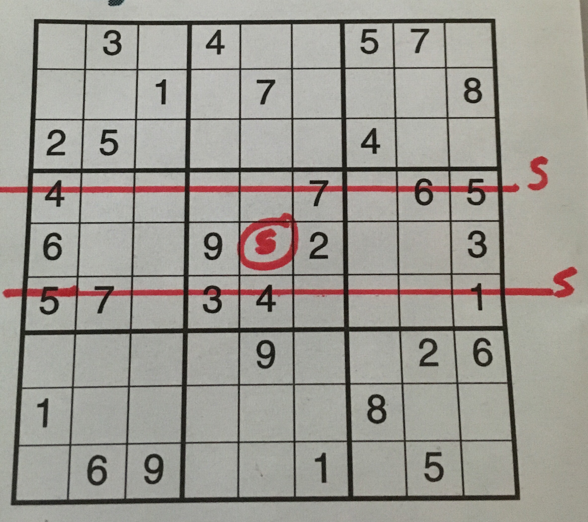
Sudoku is often held up as an example of a puzzle that mathematicians are particularly good at – infact you need no mathematical knowledge to solve sudoku problems, which require only logical thinking. There are many heuristic methods used to solve Sudoku puzzles by hand (see this book for some). A common way in is to “look for pairs” like in the picture below: There is a 5 in the 4th row and in the 6th row, we know that there must be a 5 in the 5th row; since there is already a 5 in box 4 and box 6 we can insert a 5 in indicated position.
 I must confess that I have never solved a Sudoku by hand (in fact the above is as far as I have ever gone with a Sudoku) and when I was given a book of Sudoku puzzles as a present my first thought was to write a program to solve them so I would never have to waste my time solving one by hand.
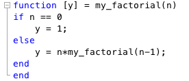
One way of solving Sudoku is to implement a recursive back-tracking procedure. Recursion is a fairly basic computer science technique where a function can call itself. The classical simple example of recursion is in the computation of the factorial function since \(n! = n \times (n-1)! \). This definition of the factorial function can be implemented in Matlab in the following way, not the call to itself in the body of the function.
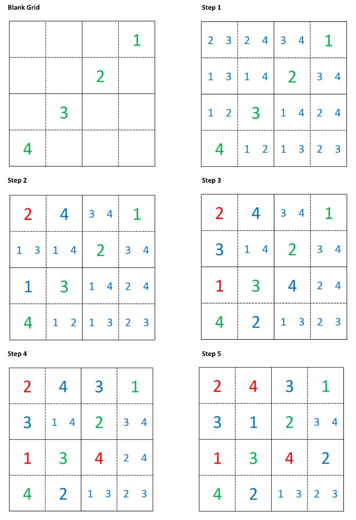
Having familiarised ourselves with the concept of recursion, lets return to solving Sudoku. An algorithm can be explained as follows:
- Read in the blank grid.
- Compute candidates for empty cells by applying the rules of sudoku.
- Fill in all singletons
- Exit if there are no candidates for any cells.
- Fill in a tentative value for an empty cell.
- Call the program recursively until the puzzle is solved.
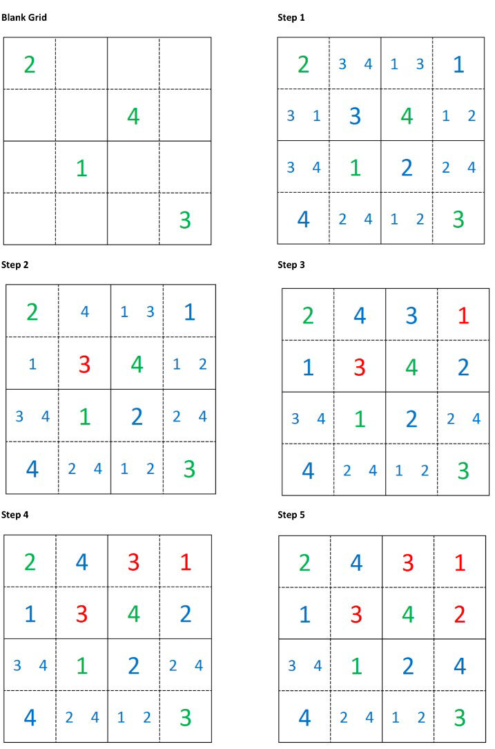
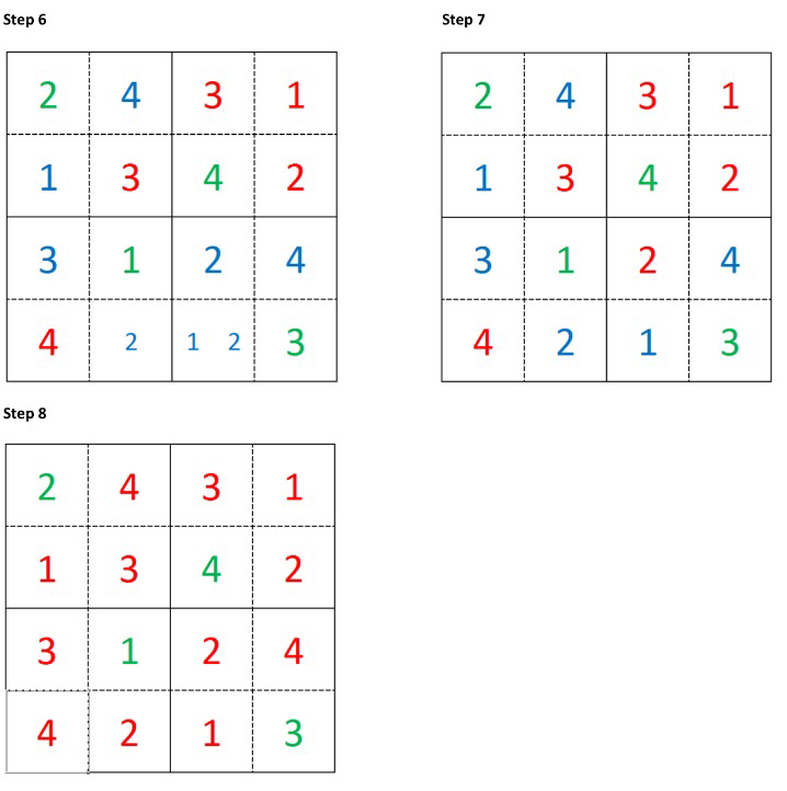
As an example consider the simpler “Shikoku” puzzle below: at each step there is a suitable singleton we can select. Thus, to solve this puzzle there is no need to fill in any tentative values and the solution is easily computed:
Sometimes there aren’t any clear singletons to choose and we have to tentatively choose a number to fill in and then recompute all the possibilities, such as the example shown below.
These examples motivate a few questions to think about
- How can we optimally choose singletons in order to compute the solution in the minimum number of steps?
- For a Shikoku, what is the minimal number of clues required for a solution to exist.
In the example above, once we have filled in one tentative value all further steps have at least one singleton we can choose from. Of course Sudoku is harder than Shidoku, and often the selection of an entry results in there being no candidates a few steps later, hence the need to go back, choose another entry and restart the solution process from that step. This can be seen nicely in the video below
The video above has been created using the Sudoku code described by Cleve Moler in his “Experiments with Matlab” book. If you are interested in learning more about the recursive backtracking approach to solving Sudoku I would encourage you to read the appropriate chapter and look at the MATLAB code.
Following this, Jasmina described another approach where a Sudoku problem was converted into a linear programming problem and then the power of MATLAB’s Optimization Toolbox was employed to solve the resulting problem which has linear objective functions, linear constraints and the constraint that some variables must be integers.
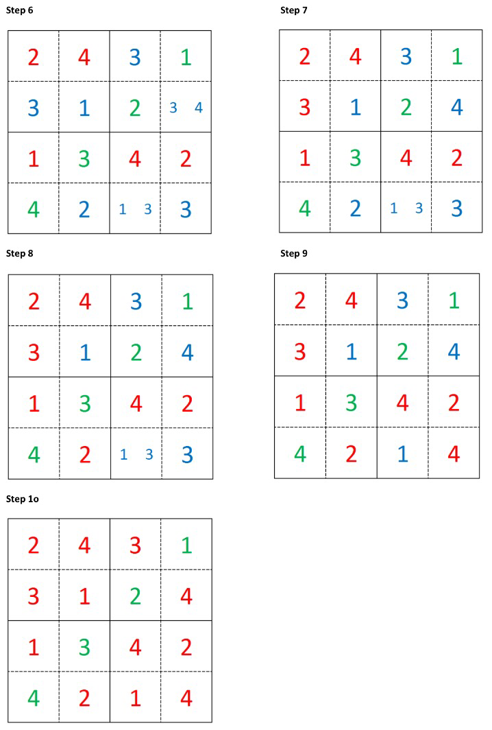
To represent Sudoku as a binary integer program the 9-by-9 grid of clues (which cells have entries) and answers into a 9-by-9-by-9 cube of binary numbers. With reference to the picture below, a clue of 5 in position (3,4) in the Sudoku problem becomes a 1 at level 5 in the cube at coordinate (3,4).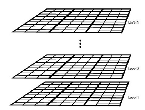
Of course at a solution we must have exactly one 1 in the stack at each grid coordinate. We can represent this mathematically by letting \(x(i,j,k)\) represent the value of the \((i,j)\)th entry at level \(k\) then we must have \(\sum_{k=1}^{9}x(i,j,k) = 1 \). We can represent the other rules of sudoku similarly, and then use a ‘black–box’ integer programming solver to solve the resulting problem. This Mathworks blogpost explains the more technical details if you are interested, it also goes on to describe an extension to Hyper-Sudoku.
The cool webcam solver we demonstrated makes use of the MATLAB Image Processing and Computer Vision toolboxes, and is similar to the demonstration shown in this video. You can also download the code at this link.
The Monty-Hall Problem
The Monty-Hall Problem is a classic problem in probability that causes a lot of confusion. This Numberphile video explains the problem very well:
This problem is often used as an exercise in the Statistics S1 module, for example, this question taken from the current Edexcel S1 text book.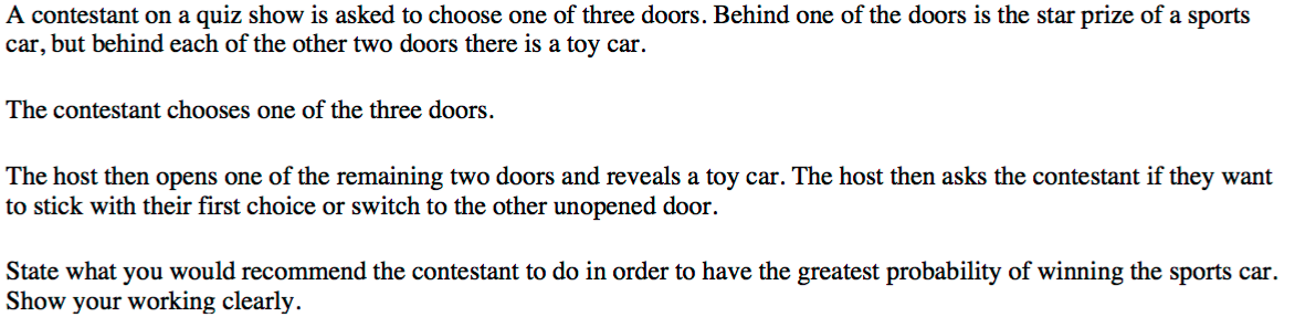
Before looking at the mathematically correct approach to this problem making use of conditional probabilities and Baye’s theorem we discussed the naive approach resulting in the diagram below 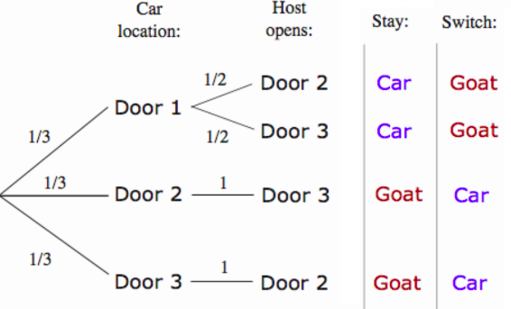
Of course without the probabilities at the end of each branch being shown this diagram backs up the a naive intuition that it makes no difference to switch – there would be a 50% chance of winning if you stay or switch.
Working through the mathematics, we instead see that the probability of winning if you switch is actually \(2/3\).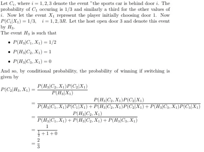
Probability is notoriously counter-intuitive and the Monty-Hall Problem is a fantastic demonstration of this. Even when shown the mathematics, many people fail to be convinced. The aim of this part of our workshop was to demonstrate how easy it is to use MATLAB to generate some simulations of the situation and quickly calculate the proportion of those where you win by switching.
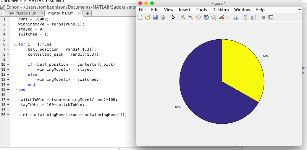
Jasmina live coded the following simulation in a couple of minutes during the session – I’m always impressed by live coding as it is so easy for things to go wrong.
This demonstration showed how easy (and quick) it is create a MATLAB file that demonstrates the Monty Hall problem and hopefully convinces even those sceptical that it is indeed better to switch.
We hope our session gave you lots to think about, please don’t hesitate to contact us if you have any questions.