Yesterday I went to an Intermediate Geogebra course at the Geogebra Institute of Sheffield run by Mark Dabbs. It was really good, and I have picked up lots of things I hadn’t realised (but probably should have done). For example, the fact that the input bar can be moved to the top of the screen so that students can more easily see it when projected onto a screen. Or that it is possible to adjust properties of many objects by just highlighting them.
I have lots of ideas of Geogebra things to do, which I’m sure I will post on here as I do them, but I thought I’d quickly share a trick (I’m sure some of you already do this) that gets rid of a little niggle of mine.
When teaching circle theorems I think it is nice to let them have a bit of time to discover them for themselves. With Geogebra you can easily create dynamic worksheets for them to explore. I’ve had a few sheets like the one below for demonstrating the “angle subtended at the centre” theorem
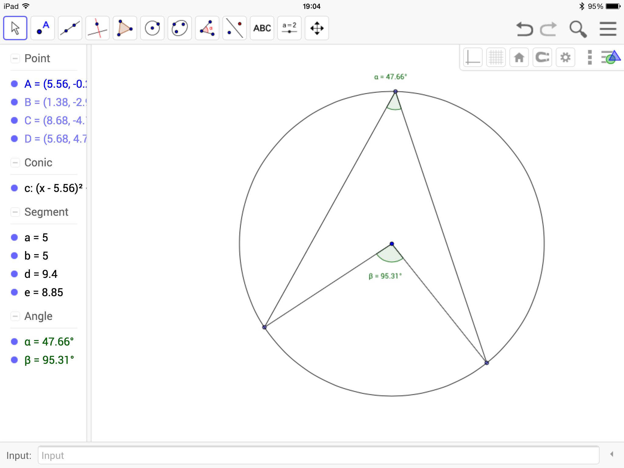
The angle at the centre is obviously meant to be twice the angle at the circumference but \( 2 \times 47.66 = 95.32 \) which is not \(95.31 \). Of course this is just an artefact of the rounding done to represent the angle to two decimal places, but it does distract from what I am hoping the students will spot. This could prompt a nice discussion about rounding errors and limits of accuracy, and of course could be mitigated somewhat by disiplaying more decimal places. But, I had always thought it would be nice if I could restrict the angle at the centre to prevent this from happening – which it turns out is easy to do. Using GeoGebra’s Sequence command (which behaves much like a for loop in a conventional programming language), we can generate a set of points around the circle such that the angle at the centre is either a whole number or a multiple of a half. This means that the angle at the edge will always be exactly represented in the two decimal places restriction.
 Once the circle with centre A has been created (by default it is given the name c), I placed one point on the circumference, call it A’ say with the command
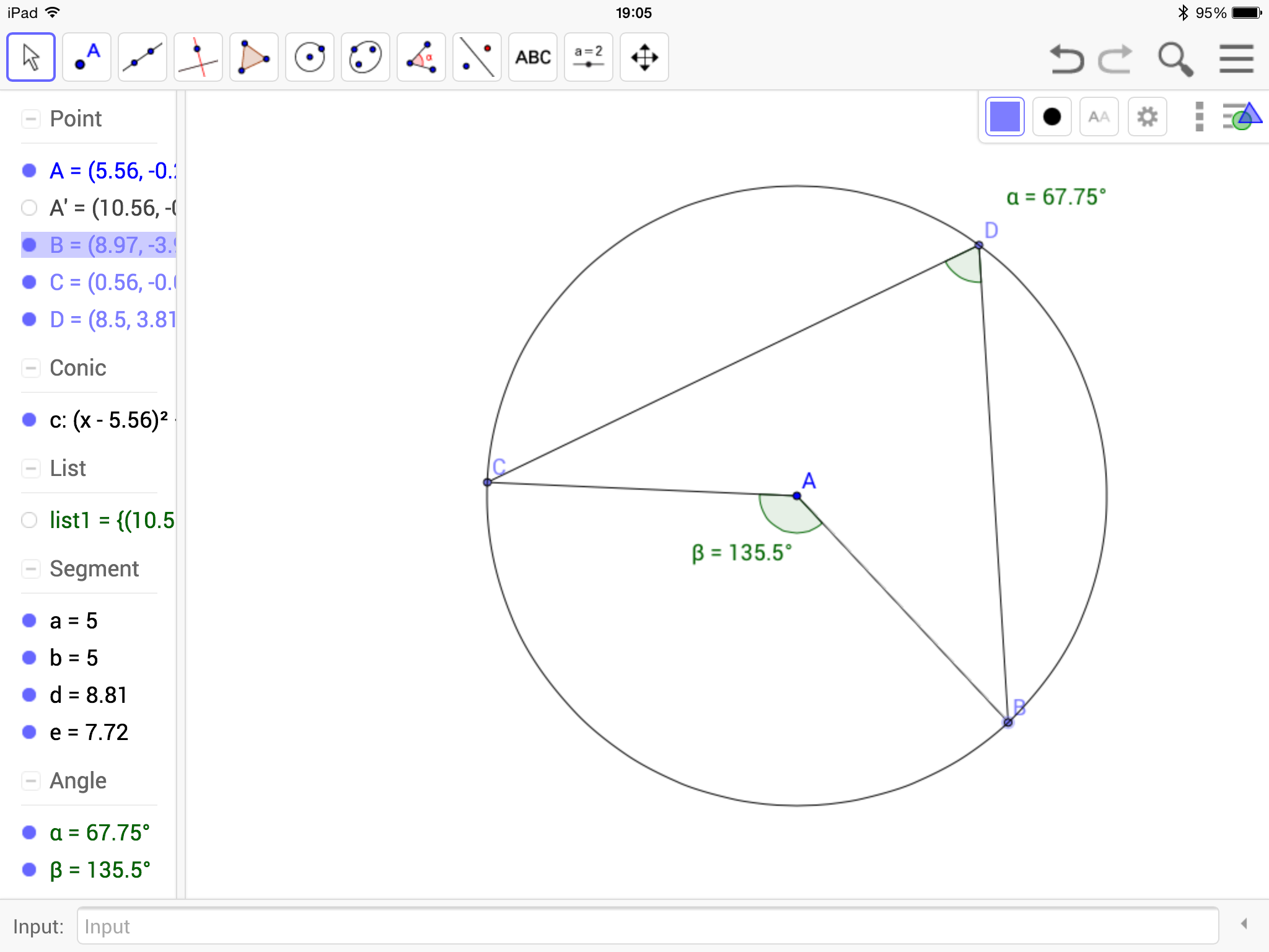
[code] A + (Radius[ c],0] [/code]. I then rotated this single point around the circle in increments of 0.5 degrees using the command [code] Sequence[Rotate[A’,kº,A],k,1,360,0.5] [/code]. This rotates the point A’ about the centre of the circle by k degrees in increments of 0.5 degrees, creating a list of points, which by default is named list1. Then you need to hide the points around the circle from the graphics view, before creating three points B,C and D on the circumference. Once you have added in the appropriate line segments the angle can be added in using the angl tool. The final step is to redefine the definition of the points B, C and D from [code] Point[ c] [/code] to [code] Point[list1] [/code] as shown below in the screen shot from the iPad app – it is much easier to do this in the desktop version.
I have hosted both versions of these basic applets on my website here.
I really would recommnd that anyone who likes using GeoGebra to attend one of Mrk’s courses, it was a great way to spend a few hours and I am hoping to go to the advanced course in July.